TensorFlow Neural Network Playground: Complete Guide & Tutorial

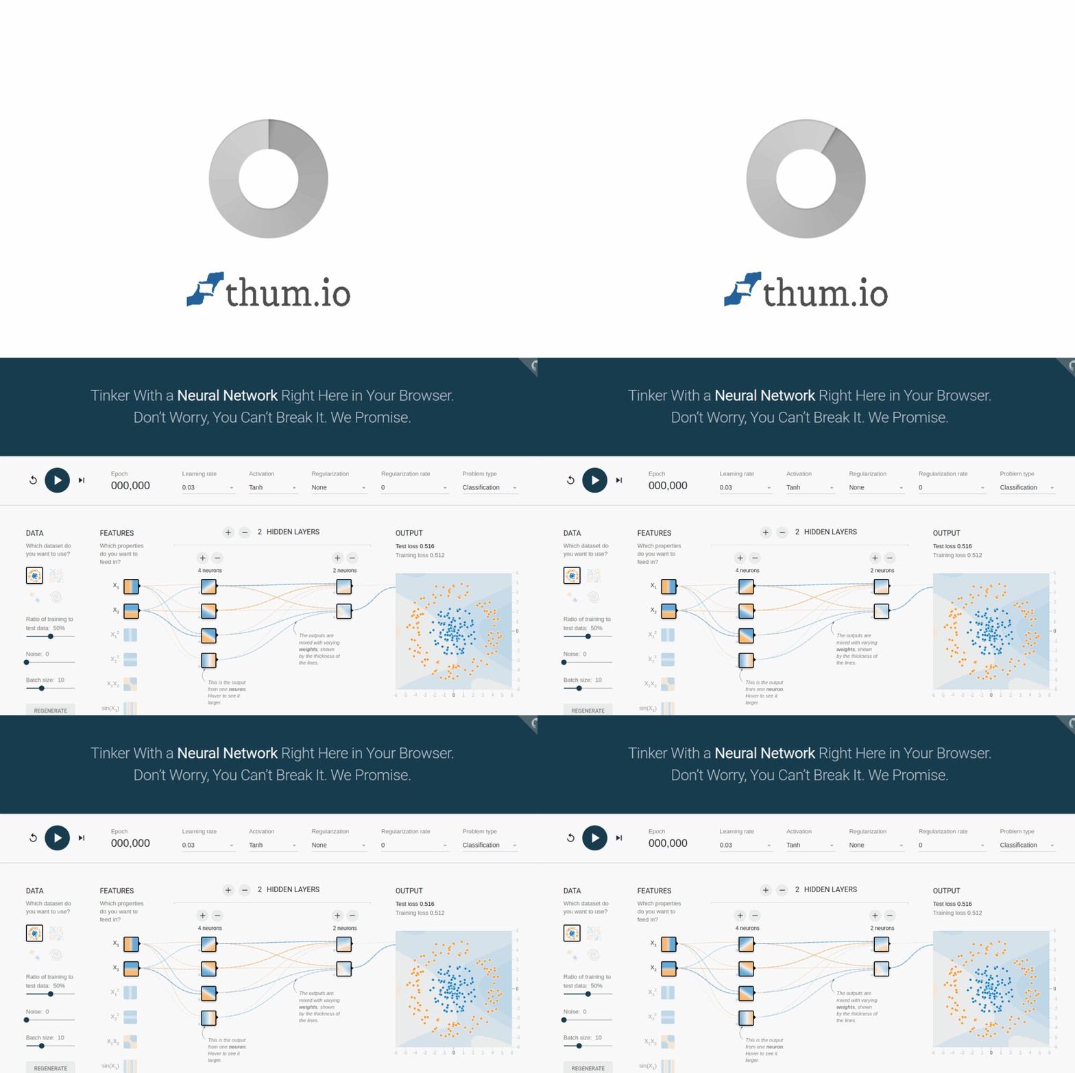
Introduction to the TensorFlow Neural Network Playground

The TensorFlow Neural Network Playground is a free, interactive web-based tool that allows you to build, train, and visualize a neural network directly in your browser without writing a single line of code. Created by the TensorFlow team, this playground is designed to demystify how neural networks learn by giving you hands-on control over every major parameter.

Whether you are a complete beginner trying to understand machine learning concepts or an experienced practitioner looking to quickly test an idea, the Playground provides an intuitive visual environment. You can adjust the learning rate, change activation functions, add regularization, modify the network architecture, and even edit individual neuron weights. The tool then shows you real-time feedback on how these changes affect training and test loss, along with color-coded predictions.

Because everything runs in your browser at the URL https://playground.tensorflow.org/, there is no software to install, no datasets to download, and no setup required. You simply open the page and start experimenting immediately.

Getting Started

Accessing the Tool

Open your preferred web browser (Chrome, Firefox, Edge, or Safari all work well). Navigate to https://playground.tensorflow.org/. The page will load instantly, presenting you with the main interface. No account creation or login is needed.

Understanding the Interface Layout

When the page loads, you will see several key areas:

• Left Panel (Data & Features): This is where you choose the dataset, the type of problem (classification or regression), and which input features to use.
• Center Panel (Network Visualization): This shows a diagram of your neural network, including input neurons, hidden layers, and output neurons. The connections between neurons are color-coded to show the weight values.
• Right Panel (Output & Loss): This displays the training and test loss over time, along with a color-coded output visualization that shows how the network is classifying or predicting data points.
• Top Controls: Here you find buttons to play/pause training, reset the network, and adjust the learning rate, activation function, regularization, and other parameters.

Your First Experiment

To get started quickly, leave all default settings as they are. You will see a classification dataset with two classes (blue and orange dots). Click the Play button (the triangle icon) located at the top-left of the interface. The network will begin training immediately, and you will see the loss values drop and the decision boundary change in the output panel. Watch for about 30 seconds, then click the Pause button (the double vertical bars) to stop training. You have just trained your first neural network.

Key Features

Adjustable Learning Rate

The learning rate controls how much the network adjusts its weights after each batch of training data. A high learning rate means larger adjustments, which can lead to faster learning but also instability. A low learning rate means smaller, more careful adjustments, which can be more stable but slower. The Playground lets you slide this value from 0.0001 to 10, and you can observe the effect on the loss graph in real time.

Activation Functions

Activation functions introduce non-linearity into the network, allowing it to learn complex patterns. The Playground offers several choices:

• ReLU (Rectified Linear Unit): Outputs the input directly if positive, otherwise outputs zero. Very popular in modern networks.
• Tanh (Hyperbolic Tangent): Squashes values between -1 and 1, centered around zero.
• Sigmoid: Squashes values between 0 and 1, often used for binary classification outputs.
• Linear: No activation, simply passes the weighted sum through unchanged.

You can apply different activation functions to each hidden layer by clicking on the layer in the network diagram.

Regularization

Regularization helps prevent overfitting, where the network memorizes the training data instead of learning general patterns. The Playground supports two types:

• L1 Regularization (Lasso): Adds a penalty proportional to the absolute value of the weights, encouraging sparse networks with many zero weights.
• L2 Regularization (Ridge): Adds a penalty proportional to the square of the weights, encouraging small but non-zero weights.

You can adjust the regularization rate (lambda) to see how it affects the decision boundary and the loss values.

Network Architecture

You can add or remove hidden layers and change the number of neurons in each layer. The Playground allows up to several hidden layers, each with a configurable number of neurons. This lets you experiment with shallow versus deep networks and observe how depth affects learning capability.

Interactive Neuron Weight and Bias Editing

One of the most educational features is the ability to click on any connection between neurons and manually adjust its weight. You can also click on a neuron itself to edit its bias term. This gives you direct insight into how individual parameters influence the network’s output.

Real-Time Visualization of Training and Test Loss

As the network trains, two lines are plotted on a graph: one for training loss (how well the network performs on the data it is learning from) and one for test loss (how well it performs on unseen data). The gap between these two lines is a strong indicator of overfitting or underfitting.

Multiple Datasets and Problem Types

The Playground includes several built-in datasets:

• Circle: A classification problem with concentric circles.
• Exclusive Or (XOR): A classic non-linearly separable problem.
• Gaussian: Two Gaussian distributions overlapping slightly.
• Spiral: A complex spiral pattern.
• Regression datasets: For predicting continuous values instead of categories.

You can switch between classification and regression problem types using the dropdown menu.

Color-Coded Output

The output panel uses color to show the network’s predictions. For classification, the background is shaded according to the predicted class, with darker shades indicating higher confidence. For regression, the color represents the predicted continuous value. This makes it easy to see at a glance whether the network is learning the correct pattern.

How to Use the TensorFlow Neural Network Playground

Step 1: Choose a Dataset

On the left panel, click the Data dropdown menu. Select from the available datasets: Circle, Exclusive Or (XOR), Gaussian, or Spiral. For regression, choose one of the regression options. You can also adjust the noise level and the ratio of training to test data using the sliders below the dataset selection.

Step 2: Select Input Features

Below the dataset, you will see boxes labeled X1, X2, X1², X2², X1*X2, and Sin(X1). These represent different mathematical transformations of your input data. Check or uncheck these boxes to control which features the network receives. For simple problems, X1 and X2 are usually sufficient. For more complex patterns, adding squared terms or sine functions can help the network learn faster.

Step 3: Design the Network Architecture

In the center panel, you can modify the network structure:

• Add a layer: Click the + button next to the hidden layers section.
• Remove a layer: Click the – button.
• Change the number of neurons: Click on a layer and use the slider that appears, or type a number directly.
• Change the activation function: Click on the activation function label (e.g., “ReLU”) above a layer and select a different one from the dropdown.

Step 4: Set Hyperparameters

At the top of the interface, adjust the following controls:

• Learning Rate: Drag the slider or type a value. Start with 0.01 or 0.03 for most problems.
• Activation: This sets the default activation for all layers. You can override it per layer later.
• Regularization: Choose None, L1, or L2, and set the regularization rate (lambda). Start with 0 or a very small value like 0.001.
• Regularization Rate: The strength of the regularization penalty.
• Batch Size: How many training examples the network sees before updating its weights. Smaller batches train faster but can be noisier.

Step 5: Train the Network

Click the Play button (triangle) to start training. The network will begin adjusting its weights, and you will see several things happen simultaneously:

• The loss graph on the right will start plotting training and test loss.
• The output panel will show the decision boundary evolving.
• The connections between neurons will change color (blue for positive weights, orange for negative, with intensity indicating magnitude).

You can pause training at any time by clicking the Pause button (double vertical bars). To reset the network to random weights, click the Reset button (circular arrow).

Step 6: Manual Editing (Optional but Educational)

To truly understand how neural networks work, try editing individual weights:

• Edit a weight: Click on any line connecting two neurons. A small popup will appear showing the current weight value. Type a new value and press Enter. The output will update immediately.
• Edit a bias: Click on any neuron (except input neurons). A popup will show the bias value. Change it and observe how the decision boundary shifts.

This is a powerful way to see the direct effect of individual parameters on the network’s behavior.

Step 7: Analyze the Results

After training, examine the loss graph. If the training loss is low but the test loss is high, the network is overfitting. You can try increasing regularization, reducing the network size, or adding more training noise. If both losses are high, the network may be underfitting, and you can try a larger network or more training epochs.

Switch to different datasets and repeat the process. Notice how some problems (like XOR) require a hidden layer with non-linear activation, while simple linearly separable problems can be solved with just a single output neuron.

Tips for Effective Learning and Experimentation

Start Simple

Begin with the simplest dataset (Gaussian) and a single hidden layer with just two or three neurons. Add complexity gradually. This will help you build an intuition for how each parameter affects the network before tackling more challenging problems.

Watch the Loss Curves Carefully

The training and test loss curves are your most important diagnostic tools. If the test loss starts to rise while the training loss continues to fall, you are seeing overfitting in real time. Pause training and experiment with regularization or a simpler network.

Use the Reset Button Often

Each time you change a major parameter (like the learning rate or activation function), click the Reset button to start training from scratch. Otherwise, you are comparing results from different starting points, which can be misleading.

Experiment with Feature Engineering

Try adding squared features (X1², X2²) or the product feature (X1*X2) to see how they help the network solve problems like the circle or XOR dataset. This demonstrates why feature engineering is so important in machine learning.

Compare Activation Functions

Train the same network on the same dataset using ReLU, Tanh, and Sigmoid activations. Notice how ReLU often trains faster but can sometimes lead to “dead neurons” (neurons that output zero for all inputs). Tanh tends to be more stable for small networks.

Understand the Role of Regularization

Train a large network (three hidden layers with many neurons) on a small dataset. You will likely see overfitting. Then add L2 regularization with a rate of 0.01 or 0.1 and retrain. Observe how the decision boundary becomes smoother and the test loss improves.

Don’t Ignore the Batch Size

Try training with a batch size of 1 (stochastic gradient descent) versus a batch size equal to the full dataset. Small batch sizes train faster per epoch but the loss curve will be noisy. Large batch sizes give smoother curves but each epoch takes longer. This is a fundamental trade-off in real-world training.

Use the Tool as a Teaching Aid

If you are learning with others or teaching, the Playground is excellent for demonstrations. You can show how a single neuron learns a linear decision boundary, then add a hidden layer to solve XOR, and finally demonstrate overfitting by adding too many neurons.

Try the Regression Datasets

Most users focus on classification, but the regression datasets are equally valuable. Switch to a regression problem and observe how the network learns to fit a continuous function. The output panel will show a color gradient instead of two colors, and the loss graph will show mean squared error instead of cross-entropy.

Save Your Configurations

The Playground does not have a built-in save feature, but you can take screenshots of your interface at different stages. Alternatively, note down the parameters you used (dataset, features, architecture, learning rate, activation, regularization) so you can reproduce your experiments later.

The TensorFlow Neural Network Playground is one of the most accessible and powerful learning tools in the machine learning ecosystem. By spending just 15 minutes experimenting with different settings, you can gain an intuitive understanding of concepts that would otherwise require months of study. Open the page, start clicking, and watch the magic of neural networks unfold before your eyes.